Waveforms

This tutorial is about understanding waveforms in DICOM datasets and covers:

• An introduction to DICOM waveforms

• Decoding and displaying Waveform Data

• Encoding Waveform Data

It’s assumed that you’re already familiar with the dataset basics.

Prerequisites

python -m pip install -U pydicom>=2.1 numpy matplotlib

conda install numpy matplotlib
conda install -c conda-forge pydicom>=2.1

References

• Waveform Module

• Waveform Explanatory Information

• Waveform Information Model

• Waveform IODs

Waveforms in DICOM

There are a number of DICOM Information Object Definitions (IODs) that contain waveforms, such as 12-Lead ECG, Respiratory Waveform and Real-Time Audio Waveform. Every waveform IOD uses the Waveform Module to represent one or more multi-channel time-based digitized waveforms, sampled at constant time intervals.

The waveforms within a dataset are contained in the items of the (5400,0100) Waveform Sequence element:

>>> from pydicom import dcmread
>>> from pydicom.data import get_testdata_file
>>> fpath = get_testdata_file("waveform_ecg.dcm")
>>> ds = dcmread(fpath)
>>> ds.SOPClassUID.name
'12-lead ECG Waveform Storage'
>>> waveforms = ds.WaveformSequence
>>> len(waveforms)
2

Each item in the sequence is a multiplex group, which is a group of related waveforms that are synchronised at common sampling frequency.

>>> multiplex = waveforms[0]
>>> multiplex.MultiplexGroupLabel
'RHYTHM'
>>> multiplex.SamplingFrequency  # in Hz
"1000.0"
>>> multiplex.NumberOfWaveformChannels
12
>>> multiplex.NumberOfWaveformSamples
10000

So the first multiplex group has 12 channels, each with 10,000 samples. Since the sampling frequency is 1 kHz, this represents 10 seconds of data. The defining information for each channel is available in the (5400,0200) Channel Definition Sequence:

>>> for ii, channel in enumerate(multiplex.ChannelDefinitionSequence):
...     source = channel.ChannelSourceSequence[0].CodeMeaning
...     units = 'unitless'
...     if 'ChannelSensitivity' in channel:  # Type 1C, may be absent
...         units = channel.ChannelSensitivityUnitsSequence[0].CodeMeaning
...     print(f"Channel {ii + 1}: {source} ({units})")
...
Channel 1: Lead I (Einthoven) (microvolt)
Channel 2: Lead II (microvolt)
Channel 3: Lead III (microvolt)
Channel 4: Lead aVR (microvolt)
Channel 5: Lead aVL (microvolt)
Channel 6: Lead aVF (microvolt)
Channel 7: Lead V1 (microvolt)
Channel 8: Lead V2 (microvolt)
Channel 9: Lead V3 (microvolt)
Channel 10: Lead V4 (microvolt)
Channel 11: Lead V5 (microvolt)
Channel 12: Lead V6 (microvolt)

Decoding Waveform Data

The combined sample data for each multiplex is stored in the corresponding (5400,1010) Waveform Data element:

>>> multiplex.WaveformBitsAllocated
16
>>> multiplex.WaveformSampleInterpretation
'SS'
>>> len(multiplex.WaveformData)
240000

If Waveform Bits Allocated is 16 and Waveform Sample Interpretation is 'SS' then the data for this multiplex consists of signed 16-bit samples. Waveform data is encoded with the channels interleaved, so for our case the data is ordered as:

(Ch 1, Sample 1), (Ch 2, Sample 1), ..., (Ch 12, Sample 1),
(Ch 1, Sample 2), (Ch 2, Sample 2), ..., (Ch 12, Sample 2),
...,
(Ch 1, Sample 10,000), (Ch 2, Sample 10,000), ..., (Ch 12, Sample 10,000)

To decode the raw multiplex waveform data to a numpy ndarray you can use the multiplex_array() function. The following decodes and returns the raw data from the multiplex at index 0 within the Waveform Sequence:

>>> from pydicom.waveforms import multiplex_array
>>> raw = multiplex_array(ds, 0, as_raw=True)
>>> raw[0, 0]
80

If (003A,0210) Channel Sensitivity is present within the multiplex’s Channel Definition Sequence then the raw sample data needs to be corrected before it’s in the quantity it represents. This correction is given by sample x Channel Sensitivity x Channel Sensitivity Correction Factor + Channel Baseline and will be applied when as_raw is False or when using the Dataset.waveform_array() function:

>>> arr = ds.waveform_array(0)
>>> arr[0, 0]
>>> 100.0
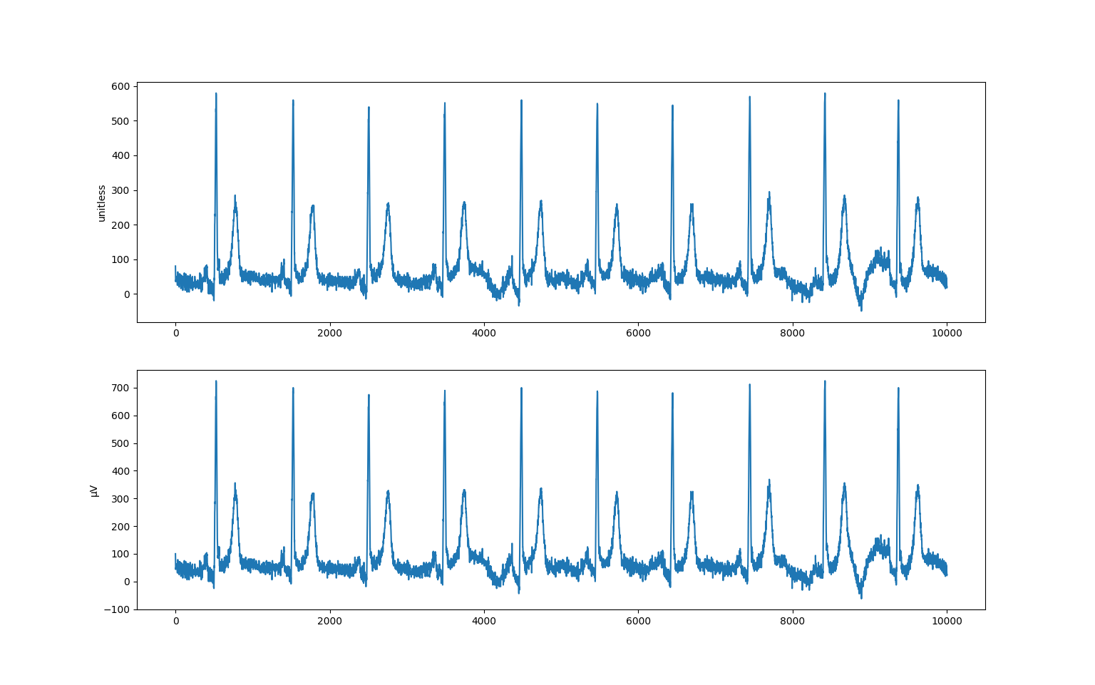
>>> import matplotlib.pyplot as plt
>>> fig, (ax1, ax2) = plt.subplots(2)
>>> ax1.plot(raw[:, 0])
>>> ax1.set_ylabel("unitless")
>>> ax2.plot(arr[:, 0])
>>> ax2.set_ylabel("μV")
>>> plt.show()

When processing large amounts of waveform data it might be more efficient to use the generate_multiplex() function instead. It yields an ndarray for each multiplex group within the Waveform Sequence:

>>> from pydicom.waveforms import generate_multiplex
>>> for arr in generate_multiplex(ds, as_raw=False):
...     print(arr.shape)
...
(10000, 12)
(1200, 12)

Encoding Waveform Data

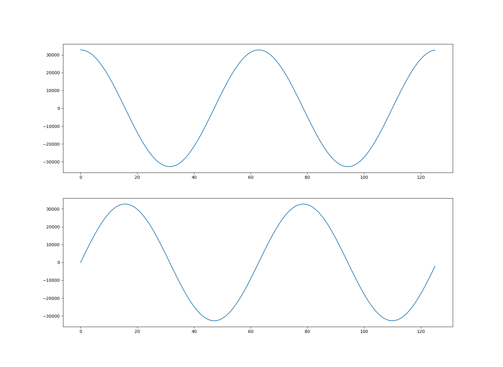
Having seen how to decode and view a waveform then next step is creating our own multiplex group. The new group will contain two channels representing cosine and sine curves. We’ve chosen to represent our waveforms using signed 16-bit integers, but you can use signed or unsigned 8, 16, 32 or 64-bit integers depending on the requirements of the IOD.

First we create two ndarrays with our waveform data:

>>> import numpy as np
>>> x = np.arange(0, 4 * np.pi, 0.1)
>>> ch1 = (np.cos(x) * (2**15 - 1)).astype('int16')
>>> ch2 = (np.sin(x) * (2**15 - 1)).astype('int16')

Next we create the new multiplex group that will contain the waveforms:

>>> from pydicom.dataset import Dataset
>>> new = Dataset()
>>> new.WaveformOriginality = "ORIGINAL"
>>> new.NumberOfWaveformChannels = 2
>>> new.NumberOfWaveformSamples = len(x)
>>> new.SamplingFrequency = 1000.0

To find out which elements we need to add to our new multiplex, we check the Waveform Module in Part 3 of the DICOM Standard. Type 1 elements must be present and not empty, Type 1C are conditionally required, Type 2 elements must be present but may be empty, and Type 3 elements are optional.

Set our channel definitions, one for each channel (note that we have opted not to include a Channel Sensitivity, so our data will be unit-less). If you were to do this for real you would obviously use an official coding scheme.

>>> new.ChannelDefinitionSequence = [Dataset(), Dataset()]
>>> chdef_seq = new.ChannelDefinitionSequence
>>> for chdef, curve_type in zip(chdef_seq, ["cosine", "sine"]):
...     chdef.ChannelSampleSkew = "0"
...     chdef.WaveformBitsStored = 16
...     chdef.ChannelSourceSequence = [Dataset()]
...     source = chdef.ChannelSourceSequence[0]
...     source.CodeValue = "1.0"
...     source.CodingSchemeDesignator = "PYDICOM"
...     source.CodingSchemeVersion = "1.0"
...     source.CodeMeaning = curve_type

Interleave the waveform samples, convert to bytes and set the Waveform Data. Since the dataset’s transfer syntax is little endian, if you’re working on a big endian system you’ll need to perform the necessary conversion. You can determine the endianness of your system with import sys; print(sys.byteorder).

We also set our corresponding Waveform Bits Allocated and Waveform Sample Interpretation element values to match our data representation type:

>>> arr = np.stack((ch1, ch2), axis=1)
>>> arr.shape
(126, 2)
>>> new.WaveformData = arr.tobytes()
>>> new.WaveformBitsAllocated = 16
>>> new.WaveformSampleInterpretation = 'SS'

And finally add the new multiplex group to our example dataset and save:

>>> ds.WaveformSequence.append(new)
>>> ds.save_as("my_waveform.dcm")

We should now be able to plot our new waveforms:

>>> ds = dcmread("my_waveform.dcm")
>>> arr = ds.waveform_array(2)
>>> fig, (ax1, ax2) = plt.subplots(2)
>>> ax1.plot(arr[:, 0])
>>> ax2.plot(arr[:, 1])
>>> plt.show()